Kafka Streams 101: Optimizing your apps for maximum performance

Last Updated: Apache Kafka version 4.0 and Responsive SDK version 0.39.0
Learning Objective: By the end of this Kafka Streams 101 lesson you will understand how your application decisions affect its overall performance and discover how to approach optimizing a Kafka Streams topology.
Quick Summary
- Break down the factors that contribute to performance in Kafka Streams
- Learn the general techniques and tradeoffs for optimizing performance
- Go through a case study based on a real world example
- Examine your options when you hit a wall and can’t meet your performance needs
Concept Overview
What even is performance?
That may sound like a dumb question, but like with any distributed system, there’s an array of distinct characteristics that may fall under the umbrella of “performance”: throughput and latency, cost and utilization, lag and availability, etc. There’s not really a one-size-fits-all definition. So to (hopefully) avoid confusion, let’s start by laying out what we mean by “performance” in the context of this blog post:
The performance of a Kafka Streams application is defined by the resources needed to meet the application requirements.
By this we just mean that this blog post is going to be focused on reducing overhead/cost for a healthy application that is already keeping up with your lag, latency, and availability needs. The first and most important thing to do with any new application is to stabilize things. We recommend checking out our blog post on sizing & capacity planning for applications at this stage. Of course, many of the techniques discussed below can also be useful if you are struggling to break even and meet the requirements from the start.
📢 Scaling up/out should be the go-to way to keep up with increasing lag or other needs — performance optimization is about what you can do to reduce the resources needed to maintain your target throughput.
With that out of the way, let’s jump in!
Performance Concepts breakdown
Kafka Streams is a complicated system, with lots of moving parts that each contribute to performance in their own way. Here we’ll break down the main factors behind an application’s profile:
Parallelism
Like any distributed system, the single most important factor is its ability to scale. Parallelism in Kafka Streams is defined by the “stream task”, the most basic unit of work that can be assigned to a StreamThread (the processing threads). The number of tasks is simply the number of subtopologies multiplied by the highest number of partitions for any source topic in that subtopology. You can use Topology#describe to get a count of the subtopologies in your application (see this section in the appendix of the upgrade guide for help).
The number of tasks represents an absolute upper limit to how far you can scale out. It’s best to think carefully about how many partitions to give new input topics for exactly this reason. But if you do find yourself scaling an application out to its maximum parallelism and still struggling to keep up with lag, fear not: you have options (some difficult, like increasing partitions, some easy — like Responsive’s Async Processor). See the final section below (To infinity & beyond: scaling past partition limits) for more on what you can do to scale beyond the limit.
Length, weight, & number of subtopologies
Since the maximum parallelism is dependent on the number of subtopologies you may be inclined to assume that more subtopologies is a good thing, but unfortunately that’s not true. One could in theory achieve higher parallelism by introducing an unnecessary repartition to split up a subtopology into two, but the added overhead of the repartition is almost never going to be worth it (unless you use this repartition to increase the downstream parallelism by expanding the partition count — more on this later)
Kafka Streams can scale pretty damn high, but the longer your topology is, the harder it will be to process records from one end to another: duh. The more subtopologies you have the more tasks there are to manage, which can put load on Kafka Streams if they aren’t spread out across multiple instances. Too many tasks on one instance can lead to memory pressure from rocksdb, as well as overhead from compactions.
The length of an individual subtopology, on the other hand, is rarely a problem for users. As long as the StreamThread can process at least one record through the subtopology for each partition/task it has assigned within the max.poll.interval.ms, it can make progress — of course if it’s taking up to 5 minutes to process a single record then you likely have other problems to deal with!
Stateful processing
This hopefully goes without saying, but generally speaking a stateful operator like aggregate or join will always be much heavier than a non-stateful operator like filter or map. The more traffic you have through your stateful operations, the harder it is to keep up with lag.
Caching & buffering
We’ll get another obvious one out of the way — caching & buffering have a huge impact on the performance of Kafka Streams applications, and are related. The built-in Streams cache (related to the statestore.cache.max.bytes config) not only reduces operations on the underlying state store, it buffers records and helps to reduce downstream traffic.
Note that the Streams record cache only buffers DSL topologies — for PAPI applications, it’s just a cache. Consider doing your own buffering by waiting to forward results until they’re complete!
De/Serialization
Last — but most certainly not least — is the overhead from de/serialization. You know: serdes and stuff. This is an unavoidable part of life in Kafka Streams, since you want to work with Java objects in your processing logic but the program needs to put things in cold hard bytes for I/O. This means any time you have to convert between application space and I/O, you’ll get de/serialization. For us, that means deserializing bytes when reading from a state store or via the consumer (for source and changelog topics), and serializing into bytes when writing to a state store or via the producer (for sink and changelog topics).
The important takeaway here is that de/serialization happens a lot — and critically, the more stateful operators and accesses, the more time spent converting between bytes and Java objects.
In sum: don’t underestimate the impact of de/serialization on Kafka Streams’ performance! Better yet, profile your application sometime and see how much time is spent in the serdes for yourself.
Configurations affecting performance
While there is unfortunately no single knob you can turn to increase performance at will (we wish!), a number of configs will directly impact the main performance metrics of throughput and latency. These are discussed below along with simple recommendations for each. Check out our sizing blog post for a larger conversation about tuning your configs.
StreamsConfig
| Config | Recommended Value | Notes |
|---|---|---|
num.stream.threads | 2x number of cores | Follow the 2x cores rule of thumb but consider experimenting to select an appropriate value for your specific application and hardware.
Can be dynamically adjusted via |
processing.guarantee | Whatever you need! | Exactly-once-semantics (EOS) has universally worse performance compared to at-least-once semantics (ALOS), but this is generally understood to be due to two indirect effects (rather than a direct impact such as the overhead from transactions):
In the end it boils down to this: only enable eos if you actually need it! You’ll have to evaluate this yourself according to your business requirements. |
statestore.cache.max.bytes | Non-zero (and consider increasing) | The bigger the cache, the greater the reduction in downstream traffic. Setting this to 0 will help you see results faster and is well-suited for testing, but this will hurt performance in applications with real traffic. The default value is only 10MB so you may also want to consider increasing this for production environments. Uses JVM heap memory, as opposed to RocksDB which uses off-heap. Make sure to leave some memory available to both. |
commit.interval.ms | Consider increasing for EOS applications | This config represents a tradeoff between throughput and latency. As with the cache size, it can make sense to set this to 0 in testing environments but this should not be used in production. Defaults to 30s in ALOS but only 100ms in EOS, which is actually a major factor in the performance drop of EOS relative to ALOS. Consider increasing it for EOS if you can afford to — evaluate within the context of your specific requirements and application (eg the more subtopologies it has, the more latency accumulates from the commit interval). |
topology.optimization | all | Be careful about changing this for existing apps, as you may need to use the application reset tool — check out our upgrade guide for details. |
num.standby.replicas | > 0 | This may not impact performance in the traditional sense, but enabling standbys is absolutely essentially for very stateful applications with a low tolerance for downtime. Of course, building up copies of the state stores means additional resource consumption in terms of both storage and bytes fetched, so like with all things: it’s a tradeoff. We just think it’s a tradeoff you should probably make. (note: may also have a small impact on throughput but this is generally negligible, and the main tradeoff is in terms of storage/IO) |
Tips & tricks for optimizing performance
So you’ve managed to scale out and/or up enough to keep up with the lag on input topics and meet your end-to-end latency requirements. Things are good, but your manager is asking you to help reduce the budget — and all the while, input traffic continues to grow alongside your company. What can you do to boost the application’s performance and minimize resources while continuing to meet your business needs?
Topology design
Probably the single biggest factor of an application’s performance is the application itself — that is, what is it actually doing? The potential savings from reviewing your topology are huge. Topology design is a complex subject so we won’t be able to cover everything here (watch out for future lessons!), but we’ll try out best to arm you with the basic principles so you can apply them to your own applications and see what there is to optimize.
Reduce repartitioning
Repartitioning is a massive source of resource usage in Kafka Streams: there’s the topics themselves, the network hop, even some overhead due to delete requests. Avoiding unnecessary repartitioning should always be top of the mind when it comes to writing new applications (but make sure to see our upgrade guide when it comes to removing repartitions from existing applications — you don’t want to lose all the data in the repartition topic!)
Here are a few tips for keeping the repartitioning to a minimum:
- always use the
topology.optimizationconfig which can reduce the number of repartition topics in certain specific situations - use the correct form of DSL operators — accidentally using the key-changing version of an operator when you don’t actually need to modify keys is a leading cause of unnecessary re partition topics. For example, prefer
mapValuesover map andgroupByovergroupByKeywhenever possible - Minimize key-changing operations between stateful operators by merging and/or moving them
Increase repartitioning
…wait, what? Isn’t this is the exact opposite of the section above? What’s going on!?
Ok, you’re right to be confused. And let us preface this by saying: introducing new repartition topics will always have overhead, most importantly increasing the end-to-end latency as well as the obvious cost of the topics themselves. Even so, it can at times make sense to manually insert your own repartition topics for reasons other than semantics.
Specifically, for the partitions! You get more of them. But we’re not just talking about the additional partitions from adding a new topic — you can insert a repartition topic to increase the partitions of everything downstream as well. With the repartition operator in the DSL you can now explicitly configure the number of partitions in a repartition topic. And since the number of partitions (and therefore tasks) of downstream subtopologies depends on the number of partitions in the upstream source topic, inserting a repartition topic with more partitions than your input topics means you get the benefit of increased parallelism for everything downstream of the new repartition. This can be a powerful option for dealing with the maximum parallelism limit, especially if you don’t control the input topics or created them with too few partitions and can’t change things now.
Filtering
Always make sure to apply any operations that reduce downstream traffic (such as filter) as soon as possible — especially if there are stateful operations downstream. For example, moving a filter from the end of a aggregation application to somewhere before the aggregate means fewer things to process and store in the heavier stateful operator, increasing overall efficiency in that operator and potentially everything else downstream of it!
Suppression
In general the actual operators in your topology should be dictated by your business needs, but if you have some flexibility in how things are processed downstream then consider suppressing intermediate results you don’t need. The Streams cache will help to buffer these and reduce traffic to following processors, but if you find your downstream applications or subtopologies being swamped by the number of unnecessary updates then suppression might be right for you!
For example, by default Kafka Streams will forward a partial result for each update to a window during a windowed aggregations. However for many use cases only the final result is important, and you can boost the effect of caching with suppression.
🖌️ Note: you can use the actual Suppress operator for in-memory suppression, or the EmitStrategy of
*ON_WINDOW_CLOSE* for an option that leverages persistent storage.
Windowing
Windowed operations such as aggregations and stream-stream joins can vary widely in performance based on the exact parameters used. Of course the ultimate deciding factor should always be your business logic rather than performance needs, but it’s worth discussing the nuances of tuning window configs for those with some flexibility in their exact requirements.
- First and foremost is the window size. Note that this may be called something different depending on the exact operator (eg
timeDifferenceMs), so we’re just using “window size” as a general term. Interestingly, the impact of window size on performance also differs depending on the operator:- for window aggregations (tumbling, hopping, and sliding windows), the bigger the window size the more efficient your application will be — assuming you have caching and/or suppression enabled. The larger the window the fewer you can fit inside a given timeframe, meaning fewer downstream updates
- for windowed joins (stream-stream joins), the smaller the window size the more efficient your application will be. This is simply because a smaller time difference means fewer joined records and thus fewer downstream results.
- Tumbling windows will generate fewer results to forward compared to hopping windows, and should be preferred unless you specifically require updates from the overlapping window segments as well.
- In the past, users who wanted sliding window semantics for windowed aggregations were instructed to model this as a hopping window with an
advanceMsof 1ms. Naturally, this leads to a very large number of updates and was considered a “last resort” tactic in the absence of native sliding window aggregations. Fortunately, sliding window aggregations were introduced to the DSL in 2.7, so any users still utilizing the previous tactic are highly recommended to upgrade to true sliding windows.
Split up independent subtopologies
Since each subtopology results in a separate set of tasks that are distributed across StreamThreads and executed independently, you can actually break up a multi-subtopology application into multiple different Kafka Streams applications for each subtopology (or subset of them). This isn’t necessarily going to boost the performance, but it can be a useful trick for a few reasons:
- Decoupling subtopologies means you can scale them independently. This is especially helpful in skewed topologies where certain subtopologies form bottlenecks for the entire application and require additional resources compared to the others.
- The more isolated the subtopologies, the easier it will be to upgrade and evolve the application topology over time. A crowded application will be more brittle.
- Limits the blast radius if you ever have to reset an application and reprocess from scratch.
Combine stateful operations to limit store accesses
Lastly, one final note for those with multiple stateful processors: never split up your stateful operations! This is mainly for you PAPI users, though some DSL users may find this helpful as well. Basically, try to do everything that happens within the same logical keyspace in a single processor. Remember: each time you access a state store, you’re not just potentially doing disk I/O, you’re forcing Streams to serialize and/or deserialize the bytes! And you don’t want to underestimate the overhead of serdes in Kafka Streams.
Which leads us to our next topic…
Serdes
Another very effective angle of attack is optimizing the way data is stored and/or manipulated. As discussed above, de/serialization and state stores/IO make up a huge part of the overall performance profile.
🔥If you want to find out just how much time is spent in de/serialization and state store accesses, try producing a flame graph! This will also give you pointers into other possible areas of improvement for your specific app.
There are a number of neat tricks you can apply to speed up your serdes, but sticking to the general principles and best practices alone should get you pretty far. Here is our advice when it comes to data modeling and serde design:
Little things add up
Your serde code is very much on the hot path, and even small, seemingly innocuous operations can really add up. This is the sort of thing that really pops with a flame graph, so try out a profiler to see if there are any easy wins before you go digging through each line of code by hand. For example, a few years ago one of our engineers was analyzing the performance of ksql, a product built on top of Kafka Streams, and found that up to 23% of the serialization time was spent just converting field names to upper case. I recommend checking out his thorough analysis here for a great example of how to approach this kind of problem.
Deserialization can be lazy
Hey, sometimes we all feel a little lazy — and deserialization is no exception. As it turns out, Kafka Streams doesn’t necessarily use the deserialized objects right away, and in some cases it may even re-serialize something without ever reading it at all. This “double serialization” can happen in foreign key joins, for example.
While this is definitely a bummer, don’t fret, because you have more control than you think: it seems to follow that if the application never uses a deserialized object then you can get away with not deserializing it all, and that’s actually true! Furthermore you can extend this to a practice called “lazy deserialization”, where instead of immediately converting the bytes to your Java object, you can return an empty object that wraps the original byte field and waits for a real access to begin the deserialization process.
You can think of it like constructing a shell that hides the serialized bytes until someone comes knocking, or in this case, until someone calls an API of that class. This only works for non-primitive types but as long as you control the Serde and data model, you can implement lazy deserialization. Check out the code below for a full example of implementing a lazy serde.
🔥 If you have large objects which are only very sparsely accessed, converting to something like flatbuffers at the beginning of your application topology may make sense to save on Serde overhead.
You don’t have to deserialize everything
Very often Kafka Streams applications will handle complex data types with values composed of many independent fields. These can even grow over time, as upstream event sources take in more and more data and new business logic gets crammed into existing applications. Unfortunately, the longer a schema grows, the worse the performance of any Kafka Streams application that depends on it. But it doesn’t have to be that way!
Many stateful operations will operate on only a field or subset of fields in the original value. A regular serde will simply deserialize the entire thing each time a record is retrieved from the state store which can mean wasting time recreating parts of the object that aren’t needed for the operation at hand, or will be dropped when forwarded. It’s a good idea to trim your schemas of unnecessary info before any stateful operations, but if you didn’t or can’t, you can simply apply a similar methodology to the lazy deserialization by only deserializing the necessary fields.
In other words, object parameters that aren’t accessed within the scope of a stateful operation can just be set to empty/null and don’t need to be deserialized at all. Just note that to do so, you’ll need to know where the useful fields are, which is why it’s so important to plan ahead by encoding any necessary metadata and versioning your schemas.
Rack awareness
Rack awareness isn’t typically thought of in the context of performance, but as we said at the top, it’s all about minimizing resources for the same baseline requirements: and cost is the resource. So how does rack awareness help you save costs, and how can you maximize the benefit from it?
Put simply: by configuring both clients and brokers with a rack.id, Kafka can ensure that clients will prefer to fetch data from partitions owned by a replica in the same rack, thus eliminating cross-AZ traffic and greatly reducing costs. There are two different strategies for realizing this benefit, which can be enabled separately for some small benefit, but should generally be enabled in combination:
- KIP-392: Allow consumers to fetch from closest replica
- Enabled by setting the broker config
replica.selector.classtoRackAwareReplicaSelector - Allows client to read from followers in the same rack when the leader has a different rack id
- Caution: can incur some per-request latency when reading from followers
- Enabled by setting the broker config
- KIP-925: Rack aware task assignment in Kafka Streams
- Enabled by setting the Streams config
rack.aware.assignment.strategy - Optimizes task assignment to match partitions to clients with the same rack id, thus improving the chance of a replica being available in the same AZ
- Enabled by setting the Streams config
Case study
To emphasize how much of a boost you can get from optimizing your application, let’s walk through a case study based on a real world example. While the improvements discussed here are specific to this individual application, the principles are generic and the approach demonstrates the kind of thing to look out for when optimizing performance. You may even find the specific use case similar to one of your own, in which case we encourage you to apply this lesson to your own code!
The Application
This case study is centered around an order batching application. A Kafka Streams user we worked with had written a custom stateful processor which stored incoming events in batches that were periodically flushed via a stream-time punctuator. In this application the input events were individual purchases, which they batched to form the output events as grouped “orders”.
This sample code demonstrates the original implementation and functionality:
private static class BatchProcessor implements Processor<String, Order, String, GroupedOrder> {

    private ProcessorContext<String, GroupedOrder> context;
    private KeyValueStore<String, OrderBatch> ordersStore;

    @Override
    public void init(final ProcessorContext<String, GroupedOrder> context) {
      this.context = context;
      this.ordersStore = context.getStateStore(PURCHASES_STORE_NAME);
      this.context.schedule(
          Duration.ofSeconds(30),
          PunctuationType.STREAM_TIME,
          this::flushReadyOrders
      );
    }

    @Override
    public void process(final Record<String, Order> newPurchase) {
      final String key = newPurchase.key();
      final long newPurchaseTimestamp = newPurchase.timestamp();
      final long newPurchaseSize = (long) newPurchase.value().amount();

      // first retrieve the current order batch for this key
      final OrderBatch oldBatch = ordersStore.get(key);

      // create an updated order batch with the new purchase
      final List<Order> updatedOrders = new ArrayList<>();
      updatedOrders.add(newPurchase.value());
      if (oldBatch != null) {
        updatedOrders.addAll(oldBatch.orders());
      }

      final long batchTimestamp = oldBatch == null ? newPurchaseTimestamp : oldBatch.timestamp();

      final OrderBatch newOrderBatch = new OrderBatch(
          updatedOrders,
          batchTimestamp,
          oldBatch == null ? 1 : oldBatch.count() + 1,
          oldBatch == null ? newPurchaseSize : oldBatch.size() + newPurchaseSize,
      );

      // flush the updated GroupedOrder if it's ready, otherwise save it in the state store
      if (shouldFlush(newOrderBatch, context.currentStreamTimeMs())) {
        final GroupedOrder ordersToForward = new GroupedOrder(updatedOrders);
        context.forward(new Record<>(key, ordersToForward, batchTimestamp));
        ordersStore.delete(key);
      } else {
        ordersStore.put(key, newOrderBatch);
      }
    }

    private static boolean shouldFlush(final OrderBatch orderBatch, final long now) {
      return ((orderBatch.timestamp() - now) > 60_000)
          || (orderBatch.count() > 50)
          || (orderBatch.size() > 1_000);
    }

    private void flushReadyOrders(final long now) {
      // iterate through all the order batches to check if any are ready to be flushed
      try (KeyValueIterator<String, OrderBatch> batches = ordersStore.all()) {
        while (batches.hasNext()) {
          final KeyValue<String, OrderBatch> kv = batches.next();
          final OrderBatch orderBatch = kv.value;
          if (shouldFlush(orderBatch, now)) {
            context.forward(new Record<>(kv.key, orderBatch, orderBatch.timestamp()));
            ordersStore.delete(kv.key);
          }
        }
      }
    }
 }
The data types used here are defined as follows:
public record Order(
    @JsonProperty("orderId") String orderId,
    @JsonProperty("customerId") String customerId,
    @JsonProperty("amount") double amount
)

public record OrderBatch (
    @JsonProperty("orders") List<Order> orders
    @JsonProperty("timestamp") long timestamp, // earliest purchase tiemstamp in batch
    @JsonProperty("count") long count, // total number of purchases
    @JsonProperty("size") long size // total purchase amount
)

public record GroupedOrder(
    @JsonProperty("orders") List<Order> orders
)
As you can see, rather than store individual events and batch them at the time of flushing, events are batched as they come in. Each key stores a list of the accumulated purchases and some metadata such as the length of the list and total size of the purchases within. When the punctuator runs, it scans through the entire store and evaluates whether to flush each batch based on the earliest timestamp in the list, the number of purchases, and the total size of the order. If these conditions are met, the order is emitted downstream, and the batch is deleted from the state store.
Now, there’s nothing inherently wrong with this approach — and it worked fine for them, for a while. But as the company grew so did their traffic, which meant increasing costs and the cold terror of the looming parallelism limit imposed by the number of partitions. They needed to take action: it was time to evaluate their application for areas of optimization.
⛔ Before we dive into the analysis of this application and highlight the inefficiencies, take a moment to consider what this application is doing and see if you can guess what the problem is!
The Problem
There are basically two distinct problems here, but they both boil down to one series issue: unnecessary de/serialization. It makes sense to tackle each of these individually however:
List format
Perhaps the first thing that caught your eye was the use of a list in the stored values, with OrderBatch being similar to the ListSerde which is one of the less common OOTB serdes (although it certainly has its place in many applications). A list format can be appropriate when the lists are short, the entries are small, or the updates are few and far between. Unfortunately, none of those were true in this case. But what exactly is the problem?
As we hinted at, it all comes down to serdes. Since Kafka Streams just sees plain bytes and reads/writes, it has no way of knowing you just want to append an input purchase to the end of a serialized — to update a list-based value with a new event you have to read the current list, add the new element to it, and then write the whole thing back to the store. That means deserializing the entire list — every single old element — and then reserializing the entire thing each time a new record arrives. That’s O(N^2) de/serializations! And that’s not even getting into the overwrite and compaction overhead.
Full scans
Second, notice the full scan in the punctuator — while it can’t always be avoided, generally speaking any time the #all API is being called you’ll have a bottleneck, so it better have a good reason for appearing. In this particular case, it made sense for them to use, but did it really need to be there?
As it turns out, no — the fact that only certain batches were being flushed and deleted while others were left alone is a pretty good sign. Keep in mind that #all is a state store access, and that means deserialization of every item you iterate over. If you don’t actually need all those items, you can save a ton of cpu time by keeping them out of the results!
Of course that’s easier said than done, and you can’t always narrow down your search enough to query only the relevant data. Fortunately in this case, we had the #shouldFlush method sitting right there, telling us what should and shouldn’t be fetched.
So: we don’t want to store purchases together in combined values, and we don’t want to read any purchases that aren’t ready to be flushed. Time to put it all together and come up with a solution:
The Solution
As you’ve probably already guessed, the first piece of the puzzle is of course breaking up the list-based values and storing individual purchases. Of course, since we know to expect more than one purchase per key, we can’t just store records as [key, purchase]. Since we also need to keep track of the purchase timestamps, we can tackle both by using a composite key formatted as "<key>.<timestamp>" .
♻️In this particular case it was guaranteed that no more than one purchase per key could exist for a given timestamp, so the format
"<key>.<timestamp>"would ensure a unique key for the purchases. You can adapt the solution for non-unique timestamps by appending a unique index to each purchase store key and adjusting the bounds of the range scan in#doFlushaccordingly.
Now that we’ve broken up the purchases, we need some way of keeping track of what’s in the current batch. At the same time, we know we want the ability to distinguish batches that are ready so we don’t have to read any purchases that won’t be flushed. Let’s tackle these two problems together with a separate metadata store and save the following info for each key: {count, total_size, first_event_time}.
Now, each time a new purchase comes in, all we have to do is store the purchase under the key×tamp and then update the count and total_size in the corresponding metadata row. Instead of deserializing and reserializing every purchase in the entire batch, we just have to de/serialize the 3-element-long metadata row and serialize only the new purchase!
The rest of the complexity is moved into the flushing logic, but it’s still pretty straightforward. Each time the punctuator is triggered, we perform a range scan over the metadata store, and use that to figure out which keys are ready to be batched and flushed. Then it’s just a matter of performing another range scan over the subset of purchases with that key (effectively a prefix scan on the purchase store) and then grouping those into an order to forward downstream.
And that’s it! The flushed purchases can be deleted from the store, and the unflushed purchases are never deserialized or even read, saving cpu and possibly disk. Take a look at the prototype below for a detailed implementation, or check it out in our examples repo.
private static class BatchProcessor implements Processor<String, Order, String, GroupedOrder> {

    private ProcessorContext<String, GroupedOrder> context;
    private KeyValueStore<String, Order> purchasesStore;
    private KeyValueStore<String, OrderMetadata> metadataStore;

    @Override
    public void init(final ProcessorContext<String, GroupedOrder> context) {
      this.context = context;
      this.purchasesStore = context.getStateStore(PURCHASES_STORE_NAME);
      this.metadataStore = context.getStateStore(METADATA_STORE_NAME);
      this.context.schedule(
          Duration.ofSeconds(30),
          PunctuationType.STREAM_TIME,
          this::flushReadyOrders
      );
    }

    @Override
    public void process(final Record<String, Order> newPurchase) {
      final String key = newPurchase.key();
      final long newPurchaseTimestamp = newPurchase.timestamp();
      final long newPurchaseSize = (long) newPurchase.value().amount();

      // first store the purchase under the key+timestamp
      purchasesStore.put(storedKey(key, newPurchaseTimestamp), newPurchase.value());

      // next, we need to look up and update the tracked metadata for this key
      final OrderMetadata orderMetadata = metadataStore.get(key);

      final OrderMetadata newOrderMetadata =
          orderMetadata == null
              ? new OrderMetadata(newPurchaseTimestamp, 1, newPurchaseSize)
              : new OrderMetadata(
                  orderMetadata.timestamp(),
                  orderMetadata.count() + 1,
                  orderMetadata.size() + newPurchaseSize
              );

      // check if the key's purchases are ready to be batched and flushed,
      // otherwise just overwrite the metadata row with the new info
      if (shouldFlush(newOrderMetadata, context.currentStreamTimeMs())) {
        doFlush(key, newOrderMetadata.timestamp());
      } else {
        metadataStore.put(key, newOrderMetadata);
      }
    }

    private void flushReadyOrders(final long now) {
      // iterate through all the metadata rows and check whether the purchases
      // for each key are ready to be batched and flushed
      try (KeyValueIterator<String, OrderMetadata> range = metadataStore.all()) {
        while (range.hasNext()) {
          final KeyValue<String, OrderMetadata> kv = range.next();
          final OrderMetadata orderMetadata = kv.value;
          if (shouldFlush(orderMetadata, now)) {
            doFlush(kv.key, orderMetadata.timestamp());
          }
        }
      }
    }

    private void doFlush(final String key, final long batchTimestamp) {
      try (
          KeyValueIterator<String, Order> range = purchasesStore.range(
              storedKey(key, 0),
              storedKey(key, Long.MAX_VALUE)
          )
      ) {
        final GroupedOrder groupedOrder = new GroupedOrder(new ArrayList<>());

        while (range.hasNext()) {
          final KeyValue<String, Order> kv = range.next();
          purchasesStore.delete(kv.key);
          groupedOrder.orders().add(kv.value);
        }

        context.forward(new Record<>(key, groupedOrder, batchTimestamp));
      }

      // make sure to delete from the metadata store once the key is fully flushed
      metadataStore.delete(key);
    }

    private static boolean shouldFlush(final OrderMetadata orderMetadata, final long now) {
      return ((orderMetadata.timestamp() - now) > 60_000)
          || (orderMetadata.count() > 50)
          || (orderMetadata.size() > 1_000);
    }

    private static String storedKey(final String key, final long ts) {
      return "%s.%d".formatted(key, ts);
    }
}
The data types used in the solution are defined as follows:
public record Order(
    @JsonProperty("orderId") String orderId,
    @JsonProperty("customerId") String customerId,
    @JsonProperty("amount") double amount
)

public record GroupedOrder(
    @JsonProperty("orders") List<Order> orders
)

public record OrderMetadata(
     @JsonProperty("timestamp") long timestamp, // earliest purchase tiemstamp in batch
    @JsonProperty("count") long count, // total number of purchases
    @JsonProperty("size") long size // total purchase amount
)
While the code changes here are relatively small, the impact was powerful and immediate. The flush rate of the punctuator sped up by a full 10x, which makes sense due to the reduced IO and deserialization from skipping over batches that were not ready to be flushed.
The full effect could be seen in the “time in topic” metric that these users paid close attention to, which gauged how long new events would have to wait around in the input topic before being processed (a very useful metric for many). As the graph below displays, this showed an improvement of multiple orders of magnitude!
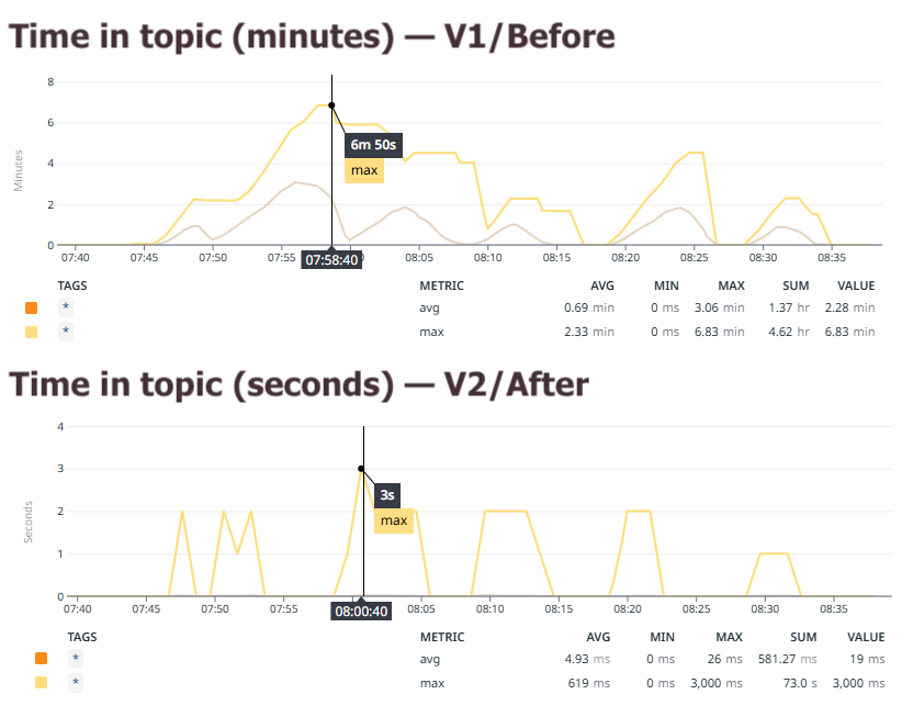
The maximum time new events had to wait in the input topic before being processed, before (top) and after (bottom) the optimization (note: the y axis is minutes in the top graph and seconds in the bottom graph)
The maximum time new events had to wait in the input topic before being processed, before (top) and after (bottom) the optimization (note: the y axis is minutes in the top graph and seconds in the bottom graph)
It’s rare to see a 100x performance improvement in most systems these days, so it just goes to show: optimizing your Kafka Streams application is no laughing matter and can have very powerful results.
To infinity & beyond: scaling past partition limits
Sometimes you do your best and it just isn’t enough: you’ve optimized every aspect of an application you can think of and scaled it up to the maximum parallelism with one task per StreamThread, but lag is still increasing. Is it just game over?
Of course not! But it may — or may not — be easy. We’ll start with the harder option and then discuss the easy one. Keep in mind these options are not mutually exclusive though: when combined the sky is truly the limit!
Increasing partitions
Did you know you can actually just…increase the number of partitions for a topic? Without having to delete and recreate it? You may not have heard of this before since it’s a relatively rare operation to perform in production. And there’s good reason for that — increasing topic partitions is risky and can be seriously harmful to your application unless performed with the utmost care and a solid understanding of the mechanism. But it is possible.
Specifically, it can be dangerous because the existing events aren’t repartitioned, leading to an initial imbalance between the old partitions and the new, empty partitions. But the real problem is that key-based partitioning typically depends on the total number of partitions, so keys that once mapped to partition N may now be mapped to partition M, and you can end up with multiple events of the same key appearing in two different partitions. Now extend this same principle to a stateful Kafka Streams application — suddenly the contents of your state stores are all mixed up and keys are scattered across the new tasks and the old ones.
Increasing partitions for stateful apps is especially tricky, but it’s not impossible. We recommend referring to the Increasing Topic Partitions section of the upgrade guide for instructions. Depending on your setup and environment you may need to introduce new topics or copy existing ones, drain the application completely, or more.
This isn’t to say that you shouldn’t ever consider raising the partition count of your input topics, and we’re not just trying to scare you for fun. We just want to emphasize that this process is difficult and requires both care and planning: it’s a last resort to raise the maximum parallelism limit and reach your throughput needs.
Async processing
So, you could go through all that to get around the partition limit — or you could try Responsive’s Async Processor.
We’ll keep this short and sweet since the topic has already been covered in depth by another blog post here. To put it shortly, async processing can give any Kafka Streams application a boost of speed by using an async thread pool to execute records from the same partition in parallel: in other words, it lets you break the maximum parallelism barrier instead of trying to raise it.
Note that the Async Processor was designed specifically to solve the performance gap with Responsive’s remote state stores and was meant to speed up processors with ~ms latencies, so it really shines with heavy processing like this and will work best for apps with state or long calls (eg RPCs) and so on. Give it a spin if you’re hitting the limits of your application — with just a few lines of code you can convert regular processors to async ones and see if this gets you to the performance you need. One thing is for sure — it’ll be easier than going through the partition raising process!
Related Metrics
| MBean | Metric | Description | Notes |
|---|---|---|---|
| kafka.consumer:type=consumer-fetch-manager-metrics,partition="{partition}",topic="{topic}",client-id="{client-id}” | records-lag | The latest lag of the partition | Make sure to check the lag on all input and repartition topics! If lag is increasing steadily or not going back down, that’s a sign to scale up. If you’re already at the maximum parallelism, you can try the above performance techniques |
| kafka.consumer:type=consumer-fetch-manager-metrics,client-id="{client-id}",topic="{topic}\” | records-consumed-rate | The average number of records consumed per second for a topic | |
| kafka.producer:type=producer-topic-metrics,client-id="{client-id}",topic="{topic}” | record-send-rate | The average number of records sent per second for a topic. | |
| kafka.streams:type=stream-thread-metrics,thread-id=([-.\w]+) | process-rate | The average number of processed records per second. | A good way to gauge overall throughput and detect a drop in performance. |
| kafka.streams:type=stream-processor-node-metrics,thread-id=([-.\w]+),task-id=([-.\w]+),processor-node-id=([-.\w]+) | record-e2e-latency-{avg/min/max} | The average end-to-end latency of a record, measured by comparing the record timestamp with the system time when it has been fully processed by the node. | Reported for source and sink/terminal nodes. Can be used to narrow in on subtopologies and detect which part of the application may be adding the most to the e2e latency. |
| kafka.streams:type=stream-thread-metrics,thread-id=([-.\w]+) | blocked-time-ns-total | The total time the thread spent blocked on kafka. |
Subscribe to be notified about the next Kafka Streams 101 lesson
Sophie Blee-Goldman
Founding Engineer